Find caves in the
terrain you've been walking past
CaveFinder reads public LIDAR elevation data to surface the quiet signatures of cave entrances — closed depressions and karst morphology — then ranks them so you know which are worth investigating.
Four steps from a box on the map to a ranked list of leads
Mark your area
of interest
Pan the map to the terrain you want to survey and enclose it in a rectangle.
Fetch the
elevation model
The best available public LIDAR is retrieved for that area and its resolution reported before scanning.
Score every
candidate site
A calibrated multi-method pipeline ranks every candidate site by how cave-like the surrounding ground looks.
Receive ranked
candidates
Candidates are ordered by confidence, plotted on the map, and exportable to your field device.
What the instrument can do
Multi-layer terrain
Hillshade, slope, aspect, curvature, and depression depth at the native resolution of the source DEM.
Geology-aware scoring
Scoring can be weighted by underlying geology where karst map data is available.
Field pins & notes
Mark candidates as visited, hit, or miss. Notes stay attached to the pin and sync across your devices.
GPX & KML export
Send a day's candidates to any handheld GPS or mapping app that accepts standard waypoint formats.
What a scan looks like
An illustrative rendering of the scan viewer: hillshaded terrain overlaid with contours, detected closed depressions, and ranked candidate pins.
Each candidate opens a feature-by-feature breakdown of the score so you can decide which leads are worth a weekend.
Calibrated against the record
CaveFinder runs over 20 scoring components across terrain-signature detection, modifier passes, and a calibrated fusion model.
Every weight is tuned against over 10,000 documented caves — so the ranking matches what cavers actually find on the ground, not what looks plausible on a hillshade.
Methodology→Turn a list of candidates into a walk you can actually do
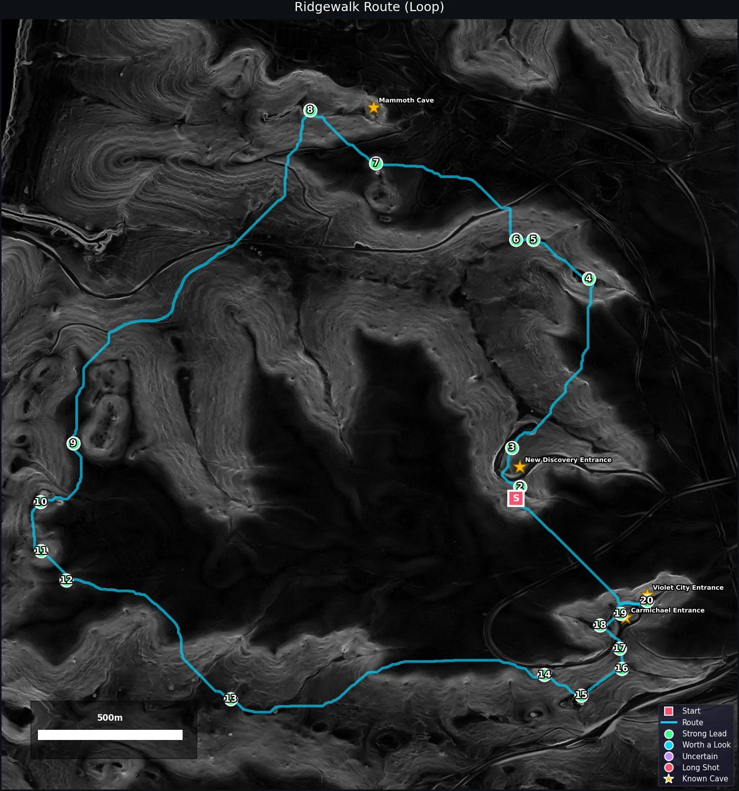
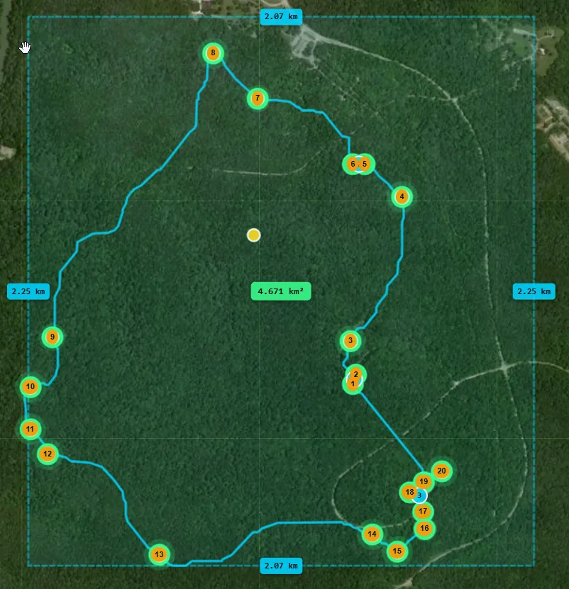
Candidates on a map are leads. Ridgewalk planning turns them into an ordered route — trailhead to last stop — optimized for the distance you want to cover, the elevation you're willing to climb, and the daylight you have.
Pick a set of candidates. Ridgewalk orders them, draws the walking line, and hands you a GPX that makes sense in the field.
Made for people who read the ground
Grotto members
and ridgewalkers
Walk a shortlist instead of a whole ridge. Built by a caver who's an NSS Director.
- GPX / KML / CSV export
- Visited & hit/miss tracking
- Known-cave overlay (public data)
- Ridgewalk Planner with PDF + GPX
Curious hikers and
weekend explorers
See what the terrain is hiding on ground you already walk. No geomorphology degree required.
- One-click simple mode
- Hillshade & slope overlays
- Saved trips
- Printable PDF with topo map
The instrument, in brief
CaveFinder works with public elevation data — no downloads, no GIS setup, no QGIS plugin. Draw a box and everything below happens automatically.
Free for most. Paid for the committed
No card. No trial timer. Three scans a week, as long as you want.
- 3 analyses per week
- All candidates, ranked & exportable
- 5 km² max scan area
- Interactive map with overlays
For cavers running real fieldwork. $59.99/yr saves 50%.
- 8 analyses per day
- 15 km² max scan area
- Ridgewalk Planner + PDF route sheet
- Field-package ZIP bundle
- Custom GeoTIFF overlay upload
- Mark as Checked field tracking
Every elevation number traces back to a public source
CaveFinder reads publicly available elevation data and overlays publicly documented cave records. The analysis math is documented on the methodology page.